Analyzing Urban Areas

This notebook shows how we can perform POI-based analysis for urban areas. Discretization of urban areas allows spatial analysis. For example, a very typical use case is to create heatmaps. You can read any spatial data that you have (e.g., real estate prices, air pollution, etc.) and start to analyze them based on the created tiles. Here we use Open Street Map to show several example use cases.

We create heatmaps of amenities based on different tessellation methods. Moreover, investigate the autocorrelation between polygons by calculating Moran’s I. In addition, different types of amenities can be extracted from POI data. For example, we visualize cafes and restaurants.

To run this notebook, in addition to tesspy, you need contextily for basemap visualization and esda, statsmodels, and libpysal for statistical and spatial analysis.

import numpy as np
import pandas as pd
import matplotlib.pyplot as plt

plt.rcParams["figure.dpi"] = 100
plt.rcParams["figure.figsize"] = (8, 8)

import geopandas as gpd
from shapely.geometry import Point
import contextily as ctx

import esda
import libpysal as lp

import statsmodels.api as sm
from scipy.stats import norm

from tesspy import Tessellation

Area

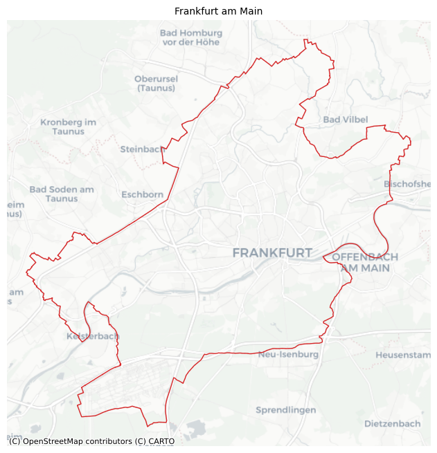
We use Frankfurt am Main in Germany as a case study. First, we get the city boundary. Then we generate different tessellations.

ffm = Tessellation("Frankfurt am Main")
ffm_polygon = ffm.get_polygon()

# visualization of area
ax = ffm_polygon.to_crs("EPSG:3857").plot(facecolor="none", edgecolor="tab:red", lw=1)
ctx.add_basemap(ax=ax, source=ctx.providers.CartoDB.Positron)
ax.set_axis_off()
ax.set_title("Frankfurt am Main", fontsize=10)
plt.show()

Tessellation

# squares
ffm_sqr_16 = ffm.squares(16)
# hexagons
ffm_hex_9 = ffm.hexagons(9)
# adaptive squares
ffm_asq = ffm.adaptive_squares(
    start_resolution=13,
    threshold=500,
    poi_categories=["shop", "building", "amenity", "office", "public_transport"],
)
# voronoi Diagrams with K-Means
ffm_voronoi_kmeans = ffm.voronoi(
    poi_categories=["shop", "building", "amenity", "office", "public_transport"],
    n_polygons=1000,
)
# voronoi Diagrams with hdbscan
ffm_voronoi_hdbscan = ffm.voronoi(
    cluster_algo="hdbscan",
    min_cluster_size=10,
    poi_categories=["shop", "building", "amenity", "office", "public_transport"],
)
# city blocks
ffm_cb = ffm.city_blocks(n_polygons=1000, detail_deg=None)

2026-02-22 17:10:24 | INFO | tesspy.tessellation | event=adaptive_squares.start start_resolution=13 poi_categories=5 threshold=500 timeout_s=300
2026-02-22 17:10:24 | INFO | tesspy.data.poi | event=poi.fetch.start poi_categories=5 timeout_s=300
2026-02-22 17:11:22 | INFO | tesspy.data.poi | event=poi.fetch.done features=164331 duration_s=57.644
/Users/siavash.saki/Personal/tesspy/tesspy/data/poi.py:118: UserWarning: Geometry is in a geographic CRS. Results from 'centroid' are likely incorrect. Use 'GeoSeries.to_crs()' to re-project geometries to a projected CRS before this operation.

  centroids = gdf.geometry.centroid
2026-02-22 17:11:22 | INFO | tesspy.data.poi | event=poi.parse.done poi_count=164331
2026-02-22 17:11:23 | INFO | tesspy.tessellation | event=adaptive_squares.subdivide resolution=14
2026-02-22 17:11:24 | INFO | tesspy.tessellation | event=adaptive_squares.subdivide resolution=15
2026-02-22 17:11:24 | INFO | tesspy.tessellation | event=adaptive_squares.subdivide resolution=16
2026-02-22 17:11:24 | INFO | tesspy.tessellation | event=adaptive_squares.subdivide resolution=17
2026-02-22 17:11:24 | INFO | tesspy.tessellation | event=adaptive_squares.done tiles=855 duration_s=59.479
2026-02-22 17:11:24 | INFO | tesspy.tessellation | event=voronoi.start cluster_algo=k-means poi_categories=5 n_polygons=1000 min_cluster_size=15 timeout_s=300
2026-02-22 17:11:24 | INFO | tesspy.tessellation | event=voronoi.cluster.start algo=kmeans
2026-02-22 17:11:29 | INFO | tesspy.tessellation | event=voronoi.polygons.create generators=1000
2026-02-22 17:11:29 | INFO | tesspy._validators | event=geometry.multipolygon.explode
2026-02-22 17:11:29 | INFO | tesspy.tessellation | event=voronoi.done polygons=1001 duration_s=5.280
2026-02-22 17:11:29 | INFO | tesspy.tessellation | event=voronoi.start cluster_algo=hdbscan poi_categories=5 n_polygons=100 min_cluster_size=10 timeout_s=300
2026-02-22 17:11:29 | INFO | tesspy.tessellation | event=voronoi.cluster.start algo=hdbscan
/Users/siavash.saki/Personal/tesspy/.venv/lib/python3.12/site-packages/sklearn/cluster/_hdbscan/hdbscan.py:722: FutureWarning: The default value of `copy` will change from False to True in 1.10. Explicitly set a value for `copy` to silence this warning.
  warn(
2026-02-22 17:12:16 | INFO | tesspy.tessellation | event=voronoi.polygons.create generators=1425
2026-02-22 17:12:17 | INFO | tesspy._validators | event=geometry.multipolygon.explode
2026-02-22 17:12:17 | INFO | tesspy.tessellation | event=voronoi.done polygons=1428 duration_s=47.563
2026-02-22 17:12:17 | INFO | tesspy.tessellation | event=city_blocks.start n_polygons=1000 detail_deg=None
2026-02-22 17:12:17 | INFO | tesspy.data.roads | event=roads.filter.selected detail_deg=None filter=['highway'~'motorway|trunk|primary|secondary|tertiary|residential|unclassified|motorway_link|trunk_link|primary_link|secondary_link|living_street|pedestrian|track|bus_guideway|footway|path|service|cycleway']
2026-02-22 17:12:17 | INFO | tesspy.data.roads | event=roads.fetch.start
2026-02-22 17:12:57 | INFO | tesspy.data.roads | event=roads.fetch.done segments=138212 duration_s=40.207
2026-02-22 17:12:57 | INFO | tesspy.tessellation | event=city_blocks.blocks.create.start
2026-02-22 17:12:59 | INFO | tesspy.tessellation | event=city_blocks.merge.start
/Users/siavash.saki/Personal/tesspy/tesspy/methods/city_blocks.py:113: UserWarning: Geometry is in a geographic CRS. Results from 'centroid' are likely incorrect. Use 'GeoSeries.to_crs()' to re-project geometries to a projected CRS before this operation.

  [blocks.geometry.centroid.x, blocks.geometry.centroid.y]
2026-02-22 17:13:04 | INFO | tesspy.tessellation | event=city_blocks.done polygons=1043 duration_s=47.734

ffm_dfs = [
    ffm_sqr_16,
    ffm_asq,
    ffm_hex_9,
    ffm_voronoi_kmeans,
    ffm_voronoi_hdbscan,
    ffm_cb,
]
titles = [
    "Squares",
    "Adaptive Squares",
    "Hexagons",
    "Voronoi Polygons (K-Means)",
    "Voronoi Polygons (HDBSCAN)",
    "City Blocks",
]

fig, axs = plt.subplots(2, 3, figsize=(15, 10))
for ax, df, title in zip(axs.flatten(), ffm_dfs, titles):
    ax.set_axis_off()
    df.plot(ax=ax, facecolor="none", edgecolor="k", lw=0.1)
    ax.set_title(f"\n{title} (n={len(df)})")

plt.tight_layout()
plt.show()

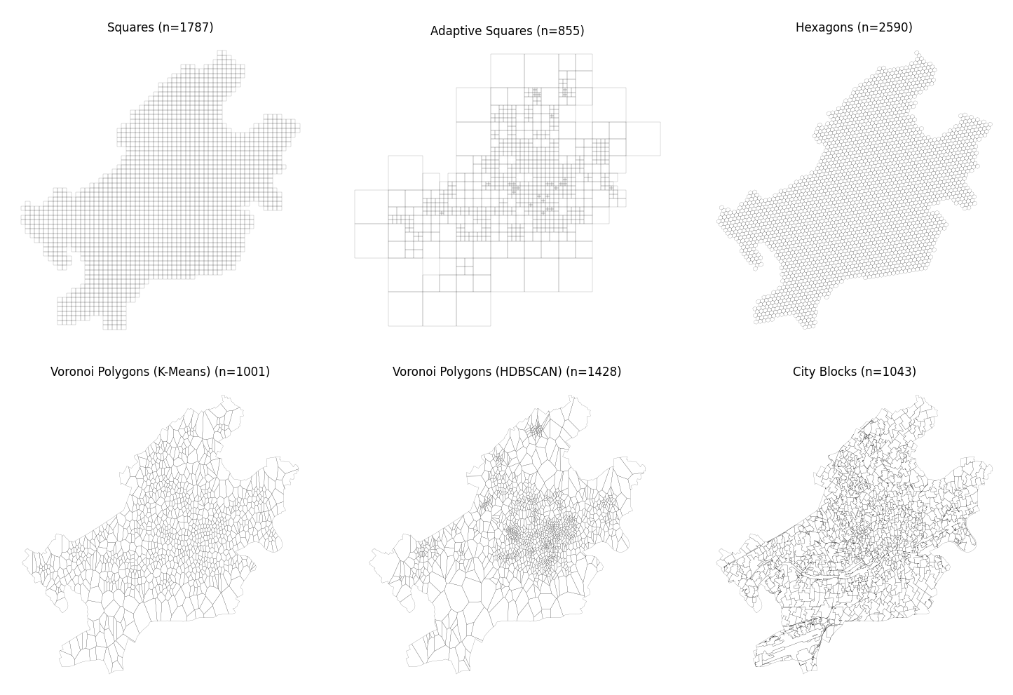
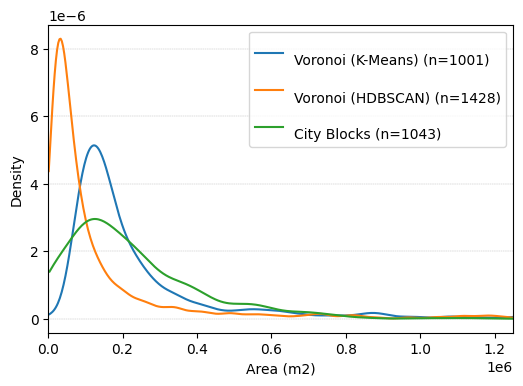
We can calculate the areas of polygons (tiles) and see how they differ between different tessellation methods. In square and hexagon methods, the area of polygons is (almost) constant. By Voronoi and city blocks, it varies. We can take a look at their histograms to investigate them.

We convert the CRS to EPSG:5243 (for Frankfurt). Using this, the coordinates are in meters, and the calculated area is in square meters.

# Calculate Areas

for df in ffm_dfs:
    df["area"] = df.to_crs("EPSG:5243").area

Here are the polygon size for squares:

ffm_sqr_16["area"].describe()

count      1787.000000
mean     153686.141422
std         307.120333
min      152971.129738
25%      153449.226805
50%      153700.251963
75%      153905.940218
max      154341.071288
Name: area, dtype: float64

Here are the polygon size hexagons:

ffm_hex_9["area"].describe()

count     2590.000000
mean     95893.520706
std         80.617912
min      95718.110703
25%      95830.679294
50%      95896.137290
75%      95960.145124
max      96061.804199
Name: area, dtype: float64

For the other Voronoi and city blocks, we create a histogram.

def trunc_dens(x):
    kde = sm.nonparametric.KDEUnivariate(x)
    kde.fit()
    h = kde.bw
    w = 1 / (1 - norm.cdf(0, loc=x, scale=h))
    d = sm.nonparametric.KDEUnivariate(x)
    d = d.fit(bw=h, weights=w / len(x), fft=False)
    d_support = d.support
    d_dens = d.density
    d_dens[d_support < 0] = 0
    return d_support, d_dens


fig, ax = plt.subplots(1, 1, figsize=(6, 4))

for df, title in zip(
    [ffm_voronoi_kmeans, ffm_voronoi_hdbscan, ffm_cb],
    ["Voronoi (K-Means)", "Voronoi (HDBSCAN)", "City Blocks"],
):

    _x, _y = trunc_dens(df["area"])
    ax.plot(_x[_x > 0], _y[-len(_x[_x > 0]) :], label=f"\n{title} (n={df.shape[0]})")
    ax.set_xlabel("Area (m2)")
    ax.set_ylabel("Density")
    ax.grid(axis="y", lw=0.3, ls="--", zorder=0)

plt.legend()
plt.xlim([0, 1.25e6])
plt.show()

POI data: Amenities

Let’s continue by taking a look at the retrieved POI data from OSM:

poi_df = ffm.get_poi_data()
poi_df.head()

	center_longitude	center_latitude	shop	building	amenity	office	public_transport
0	8.568829	50.122765	False	False	False	False	True
1	8.633793	50.153205	False	False	False	False	True
2	8.609222	50.106639	False	False	False	False	True
3	8.620979	50.107860	False	False	False	False	True
4	8.604924	50.108962	False	False	False	False	True

This dataframe contains geometry and other tags of the selected POI categories. We can take a look at the total number of each POI category in Frankfurt:

poi_df.iloc[:, -5:].sum()

shop                  4432
building            127392
amenity              28159
office                 835
public_transport      4636
dtype: int64

Let’s visualize amenities on the map:

poi_geodata = gpd.GeoDataFrame(
    data=poi_df,
    geometry=poi_df[["center_longitude", "center_latitude"]]
    .apply(Point, axis=1)
    .values,
    crs="EPSG:4326",
)

amenity_data = poi_geodata[poi_geodata["amenity"]].copy()

# visualization of area
ax = amenity_data.to_crs("EPSG:3857").plot(color="tab:blue", markersize=0.1, alpha=0.5)
ffm_polygon.to_crs("EPSG:3857").plot(ax=ax, facecolor="none", edgecolor="tab:red", lw=1)

ctx.add_basemap(ax=ax, source=ctx.providers.CartoDB.Positron)
ax.set_axis_off()
ax.set_title("Frankfurt am Main - Amenities", fontsize=10)
plt.show()

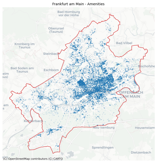
We can analyze the amenities further by querying OSM for detailed amenity types. For example, the types of amenities can be extracted. Different heatmaps for different amenity types can be provided.

import osmnx as ox

# Fetch detailed amenity features from OSM to get specific amenity types
amenity_osm = ox.features_from_polygon(
    ffm_polygon.geometry.iloc[0], tags={"amenity": True}
)
amenity_osm = amenity_osm[amenity_osm["amenity"].notna()]
amenity_data = gpd.GeoDataFrame(
    geometry=amenity_osm.geometry.centroid.values,
    crs=amenity_osm.crs,
)
amenity_data["amenity_type"] = amenity_osm["amenity"].values

/var/folders/h1/t3rj1jg93rvbrwh1ytssfg_w0000gp/T/ipykernel_75108/3521513478.py:9: UserWarning: Geometry is in a geographic CRS. Results from 'centroid' are likely incorrect. Use 'GeoSeries.to_crs()' to re-project geometries to a projected CRS before this operation.

  geometry=amenity_osm.geometry.centroid.values,

amenity_data["amenity_type"].value_counts().head(20)

amenity_type
bicycle_parking     5690
bench               4690
waste_basket        3155
parking             2972
restaurant          1325
vending_machine     1278
recycling            918
parking_space        606
kindergarten         583
cafe                 515
fast_food            513
parking_entrance     503
post_box             474
shelter              289
place_of_worship     264
doctors              259
charging_station     243
bar                  237
school               231
toilets              206
Name: count, dtype: int64

fig, axs = plt.subplots(1, 2, figsize=(10, 7))
amenity_data[amenity_data["amenity_type"] == "cafe"].to_crs("EPSG:3857").plot(
    ax=axs[0], color="tab:blue", markersize=2, alpha=0.5
)
amenity_data[amenity_data["amenity_type"] == "restaurant"].to_crs("EPSG:3857").plot(
    ax=axs[1], color="tab:blue", markersize=2, alpha=0.5
)

axs[0].set_title("Cafes")
axs[1].set_title("Restaurants")

for ax in axs.flatten():
    ax.set_axis_off()
    ffm_polygon.to_crs("EPSG:3857").plot(
        ax=ax, facecolor="none", edgecolor="tab:red", lw=1
    )
    ctx.add_basemap(ax=ax, source=ctx.providers.CartoDB.Positron)

plt.tight_layout()
plt.show()

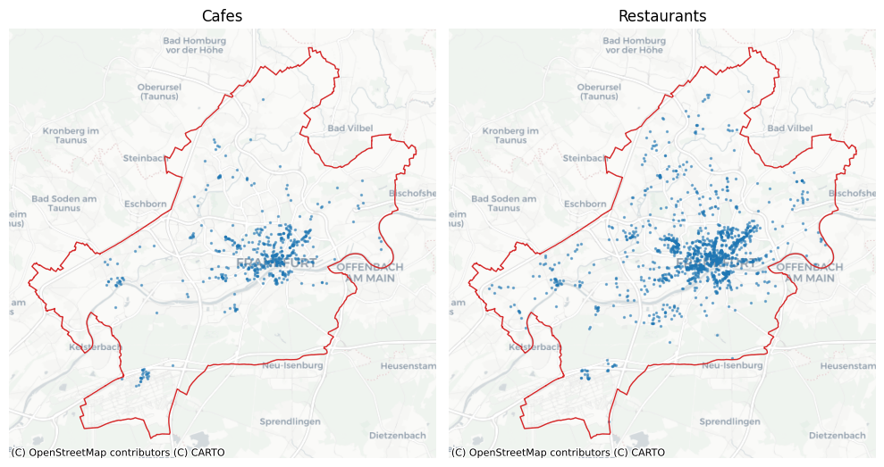
By looking at the maps, there seems to be a spatial correlation between cafes and restaurants. (This can be investigated using the tiles.)

Heatmaps for Amenities

We can use amenity to generate heatmaps based on the created polygons (tiles). First, we count amenity in each polygon for each tessellation method. Then we can visualize the resulted counts.

# adding an ID to polygons
for df in ffm_dfs:
    df.reset_index(inplace=True)
    df.rename(columns={"index": "tile_id"}, inplace=True)

# joining the amenities with the polygons
amenity_unique_qk = gpd.sjoin(
    ffm_sqr_16, amenity_data, how="left", predicate="contains"
)
amenity_unique_adaptive_qk = gpd.sjoin(
    ffm_asq, amenity_data, how="left", predicate="contains"
)
amenity_unique_hexagon = gpd.sjoin(
    ffm_hex_9, amenity_data, how="left", predicate="contains"
)
amenity_unique_voronoi_kmeans = gpd.sjoin(
    ffm_voronoi_kmeans, amenity_data, how="left", predicate="contains"
)
amenity_unique_voronoi_hdbscan = gpd.sjoin(
    ffm_voronoi_hdbscan, amenity_data, how="left", predicate="contains"
)
amenity_unique_cityblocks = gpd.sjoin(
    ffm_cb, amenity_data, how="left", predicate="contains"
)

# counting the number of amenities in each polygon
count_amenity_qk = ffm_sqr_16.merge(
    amenity_unique_qk.groupby(by="tile_id").count()["index_right"].reset_index()
)
count_amenity_adaptive_qk = ffm_asq.merge(
    amenity_unique_adaptive_qk.groupby(by="tile_id")
    .count()["index_right"]
    .reset_index()
)
count_amenity_hexagon = ffm_hex_9.merge(
    amenity_unique_hexagon.groupby(by="tile_id").count()["index_right"].reset_index()
)
count_amenity_voronoi_kmeans = ffm_voronoi_kmeans.merge(
    amenity_unique_voronoi_kmeans.groupby(by="tile_id")
    .count()["index_right"]
    .reset_index()
)
count_amenity_voronoi_hdbscan = ffm_voronoi_hdbscan.merge(
    amenity_unique_voronoi_hdbscan.groupby(by="tile_id")
    .count()["index_right"]
    .reset_index()
)
count_amenity_cityblocks = ffm_cb.merge(
    amenity_unique_cityblocks.groupby(by="tile_id").count()["index_right"].reset_index()
)

count_amenity_dfs = [
    count_amenity_qk,
    count_amenity_adaptive_qk,
    count_amenity_hexagon,
    count_amenity_voronoi_kmeans,
    count_amenity_voronoi_hdbscan,
    count_amenity_cityblocks,
]

fig, axs = plt.subplots(2, 3, figsize=(15, 10))
for ax, df, title in zip(axs.flatten(), count_amenity_dfs, titles):
    ax.set_axis_off()
    df.plot(
        ax=ax,
        column="index_right",
        lw=0.1,
        alpha=1,
        scheme="fisherjenks",
        legend=False,
        cmap="OrRd",
        edgecolor="k",
    )
    ax.set_title(f"\n{title} (n={df.shape[0]})")

plt.suptitle("Amenity count heatmap", fontweight="bold", y=1, fontsize=15)
plt.tight_layout()
plt.show()

/Users/siavash.saki/Personal/tesspy/.venv/lib/python3.12/site-packages/geopandas/plotting.py:746: UserWarning: Numba not installed. Using slow pure python version.
  binning = mapclassify.classify(
/Users/siavash.saki/Personal/tesspy/.venv/lib/python3.12/site-packages/geopandas/plotting.py:746: UserWarning: Numba not installed. Using slow pure python version.
  binning = mapclassify.classify(
/Users/siavash.saki/Personal/tesspy/.venv/lib/python3.12/site-packages/geopandas/plotting.py:746: UserWarning: Numba not installed. Using slow pure python version.
  binning = mapclassify.classify(
/Users/siavash.saki/Personal/tesspy/.venv/lib/python3.12/site-packages/geopandas/plotting.py:746: UserWarning: Numba not installed. Using slow pure python version.
  binning = mapclassify.classify(
/Users/siavash.saki/Personal/tesspy/.venv/lib/python3.12/site-packages/geopandas/plotting.py:746: UserWarning: Numba not installed. Using slow pure python version.
  binning = mapclassify.classify(
/Users/siavash.saki/Personal/tesspy/.venv/lib/python3.12/site-packages/geopandas/plotting.py:746: UserWarning: Numba not installed. Using slow pure python version.
  binning = mapclassify.classify(

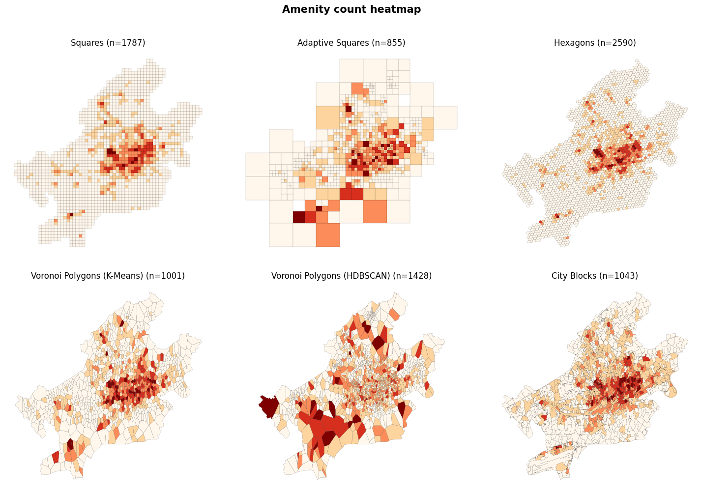
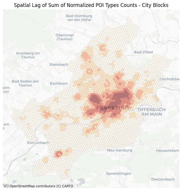
It can be seen that the most amenities are within the city center. There are many amenities near the Frankfurt airport (Southwest of Frankfurt) and also in the districts’ local centers.

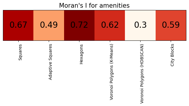
Spatial Autocorrelation: Moran’s I

At first sight, there seems to be an autocorrelation between polygons for amenities. In order to investigate the spatial autocorrelation, we can calculate Moran’s I index.

mi_values = []
for count_df in count_amenity_dfs:
    wq = lp.weights.Queen.from_dataframe(count_df)
    wq.transform = "r"
    mi = esda.moran.Moran(count_df["index_right"], wq)
    mi_values.append(mi.I)

moran_df = pd.DataFrame(dict(zip(titles, [[i] for i in mi_values])))

/var/folders/h1/t3rj1jg93rvbrwh1ytssfg_w0000gp/T/ipykernel_75108/2791682997.py:3: FutureWarning: `use_index` defaults to False but will default to True in future. Set True/False directly to control this behavior and silence this warning
  wq = lp.weights.Queen.from_dataframe(count_df)

fig, ax = plt.subplots()
ax.imshow(moran_df, cmap="OrRd", interpolation="nearest")
plt.setp(ax.get_xticklabels(), rotation=90, ha="right", rotation_mode="anchor")
plt.tick_params(axis="y", left=False, labelleft=False)
ax.set_title("Moran's I for amenities", fontsize=15)
ax.set_xticks([])
ax.set_xticks(np.arange(len(titles)), labels=titles)
for j in range(len(titles)):
    text = ax.text(
        j, 0, round(mi_values[j], 2), ha="center", va="center", color="k", fontsize=20
    )

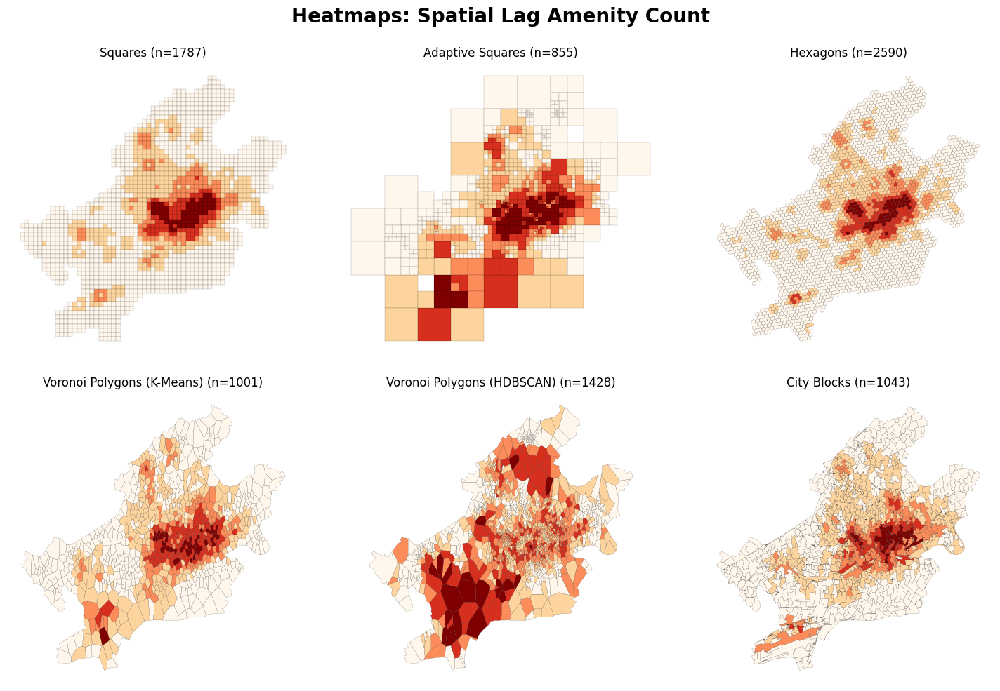
Spatial Lag

Furthermore, we can calculate spatial lags and visualize them on the map.

fig, axs = plt.subplots(2, 3, figsize=(15, 10))

for ax, count_df, title in zip(axs.flatten(), count_amenity_dfs, titles):
    wq = lp.weights.Queen.from_dataframe(count_df)
    y = count_df["index_right"]
    ylag = lp.weights.lag_spatial(wq, y)
    count_df.assign(ylag=ylag).plot(
        ax=ax,
        column="ylag",
        lw=0.1,
        alpha=1,
        scheme="fisherjenks",
        legend=False,
        cmap="OrRd",
        edgecolor="k",
    )
    ax.set_axis_off()
    ax.set_title(f"\n{title} (n={count_df.shape[0]})")

plt.suptitle("Heatmaps: Spatial Lag Amenity Count", fontweight="bold", fontsize=20)
plt.tight_layout()
plt.show()

/var/folders/h1/t3rj1jg93rvbrwh1ytssfg_w0000gp/T/ipykernel_75108/459341275.py:4: FutureWarning: `use_index` defaults to False but will default to True in future. Set True/False directly to control this behavior and silence this warning
  wq = lp.weights.Queen.from_dataframe(count_df)
/Users/siavash.saki/Personal/tesspy/.venv/lib/python3.12/site-packages/geopandas/plotting.py:746: UserWarning: Numba not installed. Using slow pure python version.
  binning = mapclassify.classify(
/var/folders/h1/t3rj1jg93rvbrwh1ytssfg_w0000gp/T/ipykernel_75108/459341275.py:4: FutureWarning: `use_index` defaults to False but will default to True in future. Set True/False directly to control this behavior and silence this warning
  wq = lp.weights.Queen.from_dataframe(count_df)
/Users/siavash.saki/Personal/tesspy/.venv/lib/python3.12/site-packages/geopandas/plotting.py:746: UserWarning: Numba not installed. Using slow pure python version.
  binning = mapclassify.classify(
/var/folders/h1/t3rj1jg93rvbrwh1ytssfg_w0000gp/T/ipykernel_75108/459341275.py:4: FutureWarning: `use_index` defaults to False but will default to True in future. Set True/False directly to control this behavior and silence this warning
  wq = lp.weights.Queen.from_dataframe(count_df)
/Users/siavash.saki/Personal/tesspy/.venv/lib/python3.12/site-packages/geopandas/plotting.py:746: UserWarning: Numba not installed. Using slow pure python version.
  binning = mapclassify.classify(
/var/folders/h1/t3rj1jg93rvbrwh1ytssfg_w0000gp/T/ipykernel_75108/459341275.py:4: FutureWarning: `use_index` defaults to False but will default to True in future. Set True/False directly to control this behavior and silence this warning
  wq = lp.weights.Queen.from_dataframe(count_df)
/Users/siavash.saki/Personal/tesspy/.venv/lib/python3.12/site-packages/geopandas/plotting.py:746: UserWarning: Numba not installed. Using slow pure python version.
  binning = mapclassify.classify(
/var/folders/h1/t3rj1jg93rvbrwh1ytssfg_w0000gp/T/ipykernel_75108/459341275.py:4: FutureWarning: `use_index` defaults to False but will default to True in future. Set True/False directly to control this behavior and silence this warning
  wq = lp.weights.Queen.from_dataframe(count_df)
/Users/siavash.saki/Personal/tesspy/.venv/lib/python3.12/site-packages/geopandas/plotting.py:746: UserWarning: Numba not installed. Using slow pure python version.
  binning = mapclassify.classify(
/var/folders/h1/t3rj1jg93rvbrwh1ytssfg_w0000gp/T/ipykernel_75108/459341275.py:4: FutureWarning: `use_index` defaults to False but will default to True in future. Set True/False directly to control this behavior and silence this warning
  wq = lp.weights.Queen.from_dataframe(count_df)
/Users/siavash.saki/Personal/tesspy/.venv/lib/python3.12/site-packages/geopandas/plotting.py:746: UserWarning: Numba not installed. Using slow pure python version.
  binning = mapclassify.classify(

Let’s take a closer look at hexagons:

f, ax = plt.subplots()

wq = lp.weights.Queen.from_dataframe(count_amenity_hexagon)
y = count_amenity_hexagon["index_right"]
ylag = lp.weights.lag_spatial(wq, y)
count_amenity_hexagon.to_crs("EPSG:3857").assign(ylag=ylag).plot(
    ax=ax,
    column="ylag",
    lw=0.1,
    alpha=0.5,
    scheme="fisherjenks",
    legend=False,
    cmap="OrRd",
    edgecolor="k",
)
ax.set_axis_off()
ctx.add_basemap(ax, source=ctx.providers.CartoDB.Positron)
ax.set_axis_off()
plt.title("Spatial Lag of Sum of Normalized POI Types Counts - City Blocks")
plt.show()

/var/folders/h1/t3rj1jg93rvbrwh1ytssfg_w0000gp/T/ipykernel_75108/673882894.py:3: FutureWarning: `use_index` defaults to False but will default to True in future. Set True/False directly to control this behavior and silence this warning
  wq = lp.weights.Queen.from_dataframe(count_amenity_hexagon)
/Users/siavash.saki/Personal/tesspy/.venv/lib/python3.12/site-packages/geopandas/plotting.py:746: UserWarning: Numba not installed. Using slow pure python version.
  binning = mapclassify.classify(